Functions in Excel. Function Wizard
Accessing the Function Wizard :Insert Function… or through the Address field while entering a formula (after entering the "=" symbol). At the first step, select a function, at the second, enter arguments into the specified fields. If any argument contains an additional function, re-access the Function Wizard only through the Address field. If, after entering the arguments of this auxiliary function, the formula does not end, click in the information field on the name of the function to which you want to go. If, after entering the function, the formula does not end, click in the information field after the already typed part of the formula and continue typing it. Press<ОК>only after completing the entire formula.
Function IF() (lab. work. SelfIf, ComplexIf) . Allows you to provide different ways to calculate the value of this function. The selection of the desired option is carried out automatically as a result of checking the condition entered into it and depending on the data entered on the Worksheet. General view of the function:
IF(Condition;ActionsIfCorrect;ActionsIfIncorrect)
According to the standard, checking the first argument should produce a TRUE or FALSE attribute.
Examples of conditions ( logical statements ):
D4>T5A5=2 AND(X2>=7;F2<=$D$8) ИЛИ(V7=$S$2;K9>=E2;J7<8)
In the last two cases, complex logical statements can be entered through auxiliary functions of the Logical category. Examples - see practical exercises.
If, given the data currently existing in the influencing cells, the Condition check shows the sign TRUE, then the algorithm from the second argument (ActionsIfCorrect) is used, otherwise - from the third (ActionsIfIncorrect).
If it is necessary to provide three or more options for calculations under different conditions, then in the first argument the condition correct for the first option is written, in the second argument this option is written, in the third argument an auxiliary function IF() is placed with the correct condition for the second option of calculations, in its this second option is written in the second argument, etc. The insertion of IF() into the third argument is repeated until all options have been sorted. Example (influencing cell A4):
IF(A4<=10;"плохо";ЕСЛИ(А4<=20;"так себе";Если(A4<=30;"нормально";"превосходно")))
If the number 7 is entered in A4, then IF() will write “bad” in its cell. If A4, for example, has 25, then the first check will produce the FALSE sign and the third argument will be selected. The function automatically switches to it when A4>=7. The IF() function in it will do an additional check and also return the FALSE sign, so its third argument will be used. Its IF() function will do one more check. This time it will show TRUE and the word "Normal" will be selected. For other examples and techniques for replacing checking one complex condition by checking several simple ones, see the practical exercises.
Construction of diagrams (lab. Work. Tables Diagrams, Coursework, Array functions and names, Population of Europe).
Diagrams are built using a table of data previously entered into the worksheet.
First stage. Sketch a diagram using the Diagram Wizard . Calling the Chart Wizard: Insert Diagram… Next 4 steps.
First – select the chart type. If the arguments are numbers or in the future it will be necessary to build a trend for forecasts, then choose Point; if the arguments are textual explanations, then any of the others. If only one indicator is depicted, and the share of each value in the total amount is important, then a Pie chart is convenient (example: revenue of different departments of a store). For several indicators on one chart, a Graph or Histogram is convenient.
Second step – set the initial data. Convenient - on the tab Rows. Button<Удалить>delete what the Master inserted himself, then<Добавить>– a blank form appears. In field Name enter the short name of the indicator for which the chart is being built (you can enter the address of the cell in which it is entered). In field Y values(or simply Values) – address of the block with indicator values. In field X values(or X-axis labels or Category labels) – block coordinates with arguments or text explanations for the indicator values. If you need to combine several indicators on one diagram, then use the button<Добавить>For each indicator, call a new form and fill it out in the same way as the first.
Third step – select the design elements of the diagram (explanatory headings, grid along the axes, position of the legend, etc.).
Fourth step – determine where to “paste” the sketch of the diagram.
Second phase. Formatting the chart and correcting parameters that were unsuccessfully set at the first stage. Basic actions:
– Changing the position and size of the entire diagram and its individual fragments: clicking on the fields or on the desired fragment, dragging the border of the frame or markers on it.
– Changing the appearance of fragments: click on the desired fragment, then Format Selected element... or right-click on the desired fragment and first command in the Context menu. You can change the fill, color, line type and thickness, axes scale, size and color of labels, etc.
– Changing the parameters specified in the first stage: clicking on any fragment of the diagram, instead of the menu Data a menu appears in the menu bar Diagram. The first 4 commands are separate steps of the Diagram Wizard; you can make changes without affecting the remaining steps of the work.
Additional features:
– adding trend lines (a line that smoothes tabular data) ;
– adding a new series of data to the chart with the same labels on the horizontal axis as for the series already included in the chart (instead of calling the command Diagram Initial data…).
Trend line. A trend is a formula (usually simple) that, within a given range of arguments, coincides well with tabular data . Creation:
Diagram Add trend line...
On the tab Type select a trend type based on samples.
On the tab Options enter a clear name for the trend, order, if necessary, forecasts beyond the available range of arguments, select a parameter Show equation in diagram.
Click<ОК>.
Typically, a trend is plotted using a Scatter chart. If a trend is plotted using a histogram, then its argument is the serial number of the data point in the table.
The trend coefficients presented in the formula on the chart are rounded to 4-5 digits. Sometimes this leads to large errors in forecasts using the trend formula. To check whether rounded factors can be used, a column (row) is added to the data table for the chart with a trend calculation for each of the table arguments. If the agreement with the tabular data is poor, then the trend is recalculated using the least squares method.
Microsoft Excel 2007 spreadsheet processor
Using Functions in Excel
1.Functions in Excel. Function Wizard. 2
2. Mathematical functions. 4
2.1.Task for independent work 1. 4
2.2.Task for independent work 2. 5
3.Statistical functions. 6
3.1.Task for independent work 3. 6
4.Logical functions. 7
4.1. Description of some logical functions. Examples. 7
4.1.1. Difficult conditions. 9
4.2. Assignment for independent work 4. 14
5.1.Task for independent work 5. 15
5.2.Task for independent work 6. 15
6.Print an Excel worksheet. 16
7. Questions for the defense of laboratory work. 16
Functions in Excel. Function Wizard
When performing calculations in spreadsheets, you often need to use functions. In the Excel package, functions are combined into categories (groups) according to their purpose and the nature of the operations performed:
* mathematical;
* financial;
* statistical;
* dates and times;
* brain teaser;
* work with the database;
* checking properties and values; ... and others.
Any function has the form:
NAME (ARGUMENT LIST)
NAME is a fixed set of characters selected from a list of functions;
ARGUMENT LIST (or just one argument) is the values on which the function performs operations. Function arguments can be cell addresses, constants, formulas, and other functions. In the case where the argument is another function, we are dealing with a nested function.
For example, the entry SUM(C7:C10;D7:D10) contains the SUM function with two arguments, each of which is a range of cells, and the entry SQRT(ABS(A2)) contains the SQRT function whose argument is the ABC function, which in its The queue argument is the address of cell A2.
Excel provides a convenient function input tool - Function Wizard. Tool Function Wizard can be called :
a) team Insert function in the tab Formulas from the group Function Library(Fig.1)
Fig.1 Team Insert function in the tab Formulas
b) team Insert function in the formula bar (Fig. 2).

Fig.2 Team Insert function in the formula bar
After the call Function Wizards a dialog box appears (Fig. 3):

Fig.3 Dialog window Function Wizards
In this window, you need to select a function category and the required function in the list below.
In the second window that appears, enter the function arguments in the appropriate fields, while for each current argument its description is displayed and the current value of this argument is displayed to the right of the argument field. When entering cell references, just select these cells in the spreadsheet (Fig. 4).

Fig.4 Mathematical function window SQRT
When a function is also used as an argument to a function, the argument function (i.e., a nested, or internal, function) should be selected by expanding the list of functions to the left of the formula bar (Fig. 5).

Fig.5 Selecting a nested (inner) function
If the required function is not in the list that appears, then you should activate the line "Other functions..." and continue working with the dialog box Function Wizard, as described above.
After entering the arguments of a nested function, you should not click on the OK button, but rather activate (click) the name of the corresponding external function in the input field of the formula bar. Those. need to go to the window Function Wizards corresponding external function. This should be repeated for all nested functions. Formulas can have up to 64 levels of function nesting.
Goal of the work:
· acquire and consolidate practical skills in creating a spreadsheet using auto-fill, auto-sum and copy capabilities;
· acquire and consolidate practical skills in using functions of the Statistical category using the Function Wizard.
Theoretical material
Formulas are expressions that are used to perform calculations. The formula always starts with an equal sign ( = ). A formula can include functions, references, operators, and constants.
A function is a standard formula that performs certain actions on values that act as arguments. Functions allow you to simplify formulas, especially if they are long or complex.
The reference points to the cell or range of worksheet cells that you want to use in the formula. You can set links to cells in other sheets of the same workbook and to other workbooks. Links to cells in other workbooks are called links.
An operator is a sign or symbol that specifies the type of calculation in a formula. There are mathematical, logical, comparison and reference operators.
A constant is a constant (not calculated) value. The formula and the result of calculating the formula are not constants.
Entering formulas from the keyboard
Formulas can be entered using the keyboard and mouse. Operators (action signs), constants (mostly numbers) and sometimes functions are entered using the keyboard. Using the mouse, select the cells to be included in the formula. Cell addresses (links) can also be entered from the keyboard, always in the English layout.
Operators (action signs) are entered using the following keys:
· addition – keyboard key + (plus);
· subtraction – keyboard key – (minus or hyphen);
· multiplication – keyboard key * (asterisk);
division – keyboard key / (fraction);
· exponentiation – keyboard key ^ (cover).
For example, when creating a formula to calculate the cost of a Bounty product in a cell D2 tables in fig. 2.1 you need to select the cell D2, enter a character from the keyboard = AT 2, enter a character from the keyboard * , left-click on the cell C2.
Rice. 2.1. Entering a formula from the keyboard
When entered from the keyboard, the formula is displayed both in the formula bar and directly in the cell (Fig. 1). Cells used in the formula are highlighted with a colored border, and references to these cells in the formula are highlighted in the same color font.
To confirm entering a formula into a cell, press a keyboard key Enter or press the button Enter(green checkmark) in the formula bar.
Creating formulas using the Function Wizard
Functions are used not only for direct calculations, but also for transforming numbers, such as rounding, looking up values, comparing, etc.
To create formulas with functions, you usually use the Function Wizard, but if you wish, functions can also be entered from the keyboard.
To create a formula, select the cell and click the button Inserting a function in the formula bar. You can also press the keyboard key combination Shift + F3.
For example, to create in a cell A11 formulas for rounding values in a cell A10 tables in fig. 2.2, you should select the cell A11.
In the dialog box Function Wizard: Step 1 of 2(Fig. 2.2) in the drop-down list Category you need to select a function category, then in the list Select function select the function and press the button OK or double-click the left mouse button on the name of the selected function.

Rice. 2.2. Selecting a function
For example, to round a number, select a category Mathematical, and the function ROUND.
If the name of the function you need is unknown, you can try to find it using keywords. To do this, after running the function wizard in the field Search function dialog box Function Wizard: Step 1 of 2(Fig. 2.3) you should enter the approximate content of the desired function and press the button Find.

Rice. 2.3. Search function
The found functions will be displayed in the list Select function. By highlighting the name of a function, you can see a brief description of it at the bottom of the dialog box. For more detailed help about the function, click on the link Help for this feature.
After selecting a function, a dialog box appears Function Arguments(Fig. 4). You must enter the function arguments in the argument fields of the dialog box. Arguments can be cell references, numbers, text, logical expressions, etc. Dialog box view Function Arguments, the number and nature of the arguments depend on the function used.
Cell references can be entered using the keyboard, but it is more convenient to select cells with the mouse. To do this, place the cursor in the appropriate field and select the required cell or range of cells on the sheet. To make it easier to select cells on a sheet, a dialog box Function Arguments can be moved or collapsed.

Rice. 2.4. Setting Function Arguments
Text, numbers, and logical expressions as arguments are usually entered from the keyboard.
Arguments can be entered into fields in any order. For example, in the table in Fig. 2.4 the value to be rounded is in the cell A10, therefore, in the field Number dialog box Function Arguments a link to this cell is provided. And in the field Number of digits argument 2 entered from the keyboard.
As a tooltip, the dialog box displays the purpose of the function, and at the bottom of the window a description of the argument in whose field the cursor is currently located is displayed.
Please note that some functions have no arguments.
When you have finished creating the function, click the button OK or keyboard key Enter.
Along with the add-on Analysis package In the practice of statistical processing, the statistical functions of Microsoft Excel can be widely used. Excel includes a library containing 78 statistical functions aimed at solving the most common problems of applied statistical analysis.
Moreover, one part of the statistical functions can be considered as a kind of elementary components of one or another superstructure mode Analysis package, the other part - as unique functions that are not duplicated in the add-on Analysis package.
However, the functions included in both the first part and the second part have independent significance and can be used autonomously when solving specific statistical problems.
The most convenient way to work with Excel statistical functions, as well as with functions from other categories, is to use the Function Wizard. When working with the Function Wizard, you must first select the function itself and then specify its individual arguments. You can launch the function wizard using the Function... command from the Insert menu, or by clicking on the function wizard button f x , or by activating the key combination Shift+F3
To make it easier to work with the wizard, individual functions are grouped thematically. Thematic categories represented in the region Category(Fig. 5). In category Full alphabetical list contains a list of all functions available to the program, K categories 10 recently used These are the ten most recently used functions. Since the user uses a limited number of functions during work, using this category you can quickly access those that are necessary in everyday work.
To define a statistical function, you must first select a category Statistical, When moving the highlight bar through the list of functions below the areas Category And Function An example will be presented illustrating how to specify the selected statistical function with brief information about it.
If the brief information is not enough, click the button in the dialog box Reference. An assistant will appear on the screen and offer assistance. Click the button Reference on the highlighted function, and the corresponding help subsystem page will be presented on the screen.
After selecting the function, click OK to proceed to the next Function Wizard dialog box, where the arguments must be specified. In this dialog box, the wizard prompts the user which arguments are mandatory (required arguments) and which are optional (optional arguments). You can set arguments in various ways, the most convenient of which are suggested by the assistant. After specifying all the function arguments, click the OK button so that the results of the function execution appear in the cell.
2. Determination of the nature of the distribution and sampling
2.1. Theoretical foundations of grouping
The results of the summary and grouping of statistical observation materials are presented in the form of tables and statistical distribution series.
Grouping is the combination of units of a statistical population into quantitative homogeneous groups in accordance with the values of one or more characteristics.
Statistical distribution series represents an ordered distribution of units of the population under study according to a certain varying characteristic. It characterizes the state (structure) of the phenomenon under study, allows us to judge the homogeneity of the population, its units of change, and the patterns of development of the observed object. The construction of distribution series is an integral part of the summary processing of statistical information.
Depending on the characteristic underlying the formation of the distribution series, there are attributive And variational distribution series. The latter, in turn, depending on the nature of the variation of the trait, are divided into discrete(intermittent) Andinterval (continuous) distribution series.
|
Example of a discrete series: Distribution of medical gowns sold by the store per month, by size.
|
Example of an interval series : Distribution of purchases at the pharmacy by amount. |
Grouping is carried out in stages. First, the approximate number of groups is determined, then the size of the interval. The first variant of the grouping is constructed, which is refined if necessary. To determine the number of groups, the Sturgess formula can be used:
where N is the population size, r– number of groups.
The size of the interval is determined by the formula:  ,
,
where x max, x min are the corresponding maximum and minimum values of the population characteristics, r– the size of the interval. The resulting result is rounded.
Equal grouping intervals are used for homogeneous populations, while unequal interval groupings are more often used for socio-economic phenomena. If the extreme value of the population units differs significantly in size from the rest, groupings with open interval boundaries are used.
The first interval is with an open lower border, the last interval is with an open upper border. The value of the first interval is assumed to be equal to the value of the next interval (no more than). The value of the last interval with an open upper border is assumed to be equal to the value of the penultimate interval.
There are absolute and relative frequency characteristics.
Absolute characteristic – frequency, shows how many times this variant of the series occurs in total. The advantage of frequency is simplicity, the disadvantage is the impossibility of comparative analysis of distribution series of different numbers.
For such comparisons, relative frequencies or frequencies, which are calculated by the formula:
 ,
,
 ,
,
where N is the population size.
This is the relative size of the structure (in terms of shape).
The sum of the frequencies is 1.

 If frequencies are expressed as percentages or ppm, their sums are equal to 100 or 1000, respectively.
In unequal interval distribution series, frequency characteristics depend not only on the distribution of series variants, but also on the size of the interval, other things being equal, expanding the boundaries of the interval leads to an increase in the fullness of the groups.
To analyze distribution series with unequal intervals, density indicators are used:
Absolute density:
where f i is the frequency, c i is the value of the interval - shows how many units in total there are per unit of value of the corresponding interval. Absolute density allows one to compare the saturation of different-sized intervals in a series. Absolute densities do not allow, however, comparison of distribution series of different abundances.
For such comparisons we use relative densities:
 , where d i – frequencies (shares), c i – values of the corresponding intervals – shows what part (share) of the population falls on a unit of value of the corresponding interval. It is most convenient to analyze distribution series using their graphical representation, which allows one to judge the shape of the distribution. A visual representation of the nature of changes in the frequencies of the variation series is given by polygon And bar chart.
Polygon used for image discrete variation series. When constructing a polygon in a rectangular coordinate system, the ranked values of the varying characteristic are plotted along the x-axis on the same scale, and the frequency scale is plotted along the ordinate axis, i.e., the number of cases in which a particular value of the characteristic was encountered. The points obtained at the intersection of abscissa and ordinate are connected by straight lines, resulting in a broken line called a frequency polygon. For example, in Fig. 6. The distribution of the number of students by academic performance and the frequency range for this distribution are shown. To construct a polygon, we will use the Microsoft Excel Chart Wizard (Graph mode).

For image interval variational series of distributions are used histograms. In this case, the values of the intervals are plotted on the abscissa axis, and the frequencies are depicted by rectangles built on the corresponding intervals. The result is a histogram - a graph in which the distribution series is presented in the form of areas adjacent to each other. To characterize distribution series, graphs of accumulated frequencies or cumulates.
Cumulates allows you to determine which part of the population has values of the characteristic being studied that do not exceed a given limit, and which part, on the contrary, exceeds this limit.
Function Wizard in Excel
Functions can be entered manually, but Excel provides a function wizard that allows you to enter them semi-automatically and with virtually no errors. To call the function wizard, you must press the button Inserting a function on the standard toolbar, run the command Insert/Function or use the keyboard shortcut . After this a dialog box will appear Function Wizard, where you can select the desired function.
Dialog window Function Wizard(Fig. 2.8) is used quite often. Therefore, we will describe it in more detail. The window consists of two interconnected lists: Category And Function. When you select one of the list items Category on the list Function a list of functions corresponding to it appears.
In Microsoft Excel, functions are divided into 12 categories. The 10 Recently Used category is constantly updated based on what features you've used recently. It is similar to stack memory: a new function you call, which is not yet on the list, will occupy the first line, thereby displacing the last function.

Rice. 2.8. Function Wizard Dialog Box
When you select a function, a brief description of it appears at the bottom of the dialog box. By pressing the button OK or key , you can call the panel of the selected function (a description of such panels is given below).
 Functions in Excel. Function Wizard. How to Use the Function Wizard to Create Formulas in Excel The Function Wizard is used to create
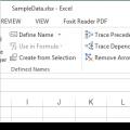 Formula bar in excel reflects
 Changing page margins in a Microsoft Word document