The formula bar in excel reflects. Creating Formulas in Excel
If you are working with an Excel worksheet that contains many formulas, it may be difficult to keep track of all of those formulas. In addition to Formula bar Excel has a simple tool that allows you to display formulas.
This tool also shows the relationship for each formula (when highlighted), so you can keep track of the data used in each calculation. Displaying formulas allows you to find the cells containing them, view them, check for errors, and print a sheet with formulas.
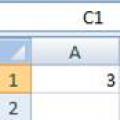
To show formulas in Excel, click Ctrl+'(apostrophe). The formulas will appear as shown in the image above. Cells associated with a formula are highlighted with borders that match the color of the references to make it easier to track the data.
You can also select the command Show Formulas(Show formulas) tab Formulas(Formula) in the group Formula Auditing(Formula Dependencies) to show formulas in Excel.

Even if the display is turned off, the formula can be viewed in Formula bar when selecting a cell. If you do not want the formulas to be visible to users of your Excel workbook, you can hide them and protect the worksheet.

The formulas will again be visible when you select cells.
The formula bar in Excel software is perhaps one of the main elements. Almost all operations are carried out with the help of it.
There are times when this line simply disappears. What to do under such circumstances? Let's figure it out.
The formula bar disappears for two reasons - either it is a software failure of Excel itself, or the settings for displaying it in the application have changed.
To get started, you can open the “View” menu and in the “Show” field, check the box next to the “Formula Bar” line.
As soon as the checkbox is checked, a line will immediately appear in the program menu. There is no need to restart the application; it is completely ready for use.

You can also enable the formula bar by changing the application settings itself. To do this, open the “File” tab and in the “Information” section select the “Options” field.

In the Excel options window that appears, you need to open the “Advanced” section and check the “Show formula bar” checkbox in the screen settings field. You can then apply the parameter changes.

If the above methods do not help you display the formula bar, it may be due to a software glitch in the application. The easiest way to fix this is to restore the program to a fully working state. To do this, open the “Start” menu and select the “Control Panel” section.

In the window that appears, select the “Uninstall a program” function.

In the list of installed programs, you need to find Excel and click on the “Change” button.
The worksheet of the book is divided by grid lines into rows and columns. Each column is assigned a specific letter, which appears as its heading. Column headings can range from A to IV (column Z is followed by AA, AZ is followed by BA, and so on up to IV). Each row is assigned an integer, which appears to the left of the worksheet grid as the row heading. Line numbers can range from 1 to 1000000.
At the intersection of a row and a column is a cell. Cells are the basic building blocks of any worksheet. Each cell occupies a place on the worksheet where you can store and display information, and has unique coordinates called a cell address or link. For example, the cell located at the intersection of column A and row 1 has address A1. The cell at the intersection of column Z and row 100 has address Z100. The selected cell is called the active cell. The address of the active cell is displayed in the name field, which is located at the left end of the formula bar.
If you're using Excel 2003 and earlier, with 256 columns and 65,536 rows, the worksheet can contain more than 16 million cells. The maximum number of usable cells is limited by the amount of memory available on the computer. Although Excel reserves memory only for cells that contain data, you are unlikely to be able to use all the cells in a single worksheet.
Scroll bars allow you to display invisible areas. The displayed area of the worksheet is called the active area (in a new Excel worksheet, these are columns A through M and rows 1 through 26). The user works with Excel in the active area of the sheet. The formula bar is used to display data entered into table cells or for direct data entry. In the formula bar, when you enter or edit data in a cell, the “Edit Formula” button is displayed.
Although you can enter information directly into a cell, using the formula bar has some advantages. When you position the pointer on the formula bar and click the mouse button, two additional buttons appear on the line: cancel and enter. When you press the enter button, Excel “captures” the information entered in the formula bar and transfers it to the worksheet. Pressing the Enter button is the same as pressing the Enter key, except that pressing Enter usually additionally activates the cell immediately below the one in which you entered data. To delete erroneously entered information, press the cancel button or the Esc key.
The cell is the main element of the worksheet of the book, the set parameters of which are:
- Numeric or data formats: general, numeric, monetary, financial, date, time, percentage, exponential, text and complementary;
- Aligning data in a cell horizontally and vertically, orienting data in a cell with a rotation of 90″ and displaying it with word wrapping or automatic width selection, or merging cells;
- Fonts for which the typeface, style, size, underline, stitch and modification are set, such as strikethrough, superscript, subscript;
- The outline of the frame of the external and internal borders of cells and ranges of cells, the type and color of lines;
- Cell fill color and pattern;
- Protect cells and hide formulas.
- Cells can be combined into ranges.
A range is a collection of adjacent cells. A range is specified by the addresses of its top left cell and bottom right cell, separated by a colon. For example A5:D8. A range, like any cell, can be given a name.
Selecting cells
To perform operations with cells or ranges, you need to select them, i.e. make active. A cell is selected by clicking the left mouse button on its field. If one cell is selected, it will become active and its address will appear in the name box at the left end of the formula bar, and a frame will appear around the cell indicating that the cell is active. A range is selected by dragging the mouse pointer over the cells included in it or by specifying the boundary cells while holding down the key Shift.
When selecting multiple ranges using the mouse, use the key Ctrl. You can also use the Add mode to select a group of ranges. After highlighting the first range, press the keys Shift+F8 to turn on the adding mode (the ADD indicator should light up in the status bar) and drag the pointer over the cells of the new range. Then click Esc or Shift+F8 to turn off add mode.
Selecting an entire column or row is done by clicking on the column or row header. The first visible cell becomes active. To select multiple adjacent columns or rows, press Shift or F8, and non-adjacent columns or rows, use the Or key/or keys Shift+F8.
Data in cells
You can enter two types of data into worksheet cells: constants and formulas. Constants fall into three main categories: numeric values, text values (also called labels, text strings, character strings, or simply text), and date and time values. In addition, Excel has two other special types of constants: boolean values and error values. Numeric values can only contain the numbers 0 through 9 and the special characters + - Ee().,$%/. The text value can contain almost any characters.
Constants and numeric values are entered from the keyboard and appear in the formula bar and in the active cell. The blinking vertical bar that appears in the formula bar and in the active cell is called the insertion point. The input is completed by pressing the Enter key or the arrow keys, Tab, Shift+Tab, Enter, Shift+Enter, after which Excel records the input and activates the adjacent cell.
When entering numeric data in Excel, the following characters have special meanings:
- If you start entering a number with a PLUS sign (+) or a minus sign (-), Excel omits the plus sign and stores the minus sign, in the latter case interpreting the entered value as a negative number.
- The symbol E or e is used when entering numbers in scientific notation. For example, Excel is interested in 1E6 as 1,000,000 (one multiplied by ten to the sixth power).
- Numeric values enclosed in parentheses. Excel interprets them as negative. (This is how negative numbers are written in accounting.) For example, the value (100) is interpreted by Excel as -100.
- You can use decimal occupied as usual. In addition, it is possible to insert a space to separate hundreds from thousands, thousands from millions, etc. When you enter numbers with spaces separating groups of digits, they appear in cells with spaces, but in the formula bar they appear without spaces. If you start entering a number with a dollar sign ($), Excel applies a currency format to the cell.
- If you end a numeric value with a percent sign (%), Excel applies the percentage format to the cell.
- If you use a slash (/) when entering a numeric value, and the character string you entered cannot be interpreted as a date, Excel treats the entered value as a fraction. For example, if you enter 115/8. Excel will display 11.625 in the formula bar and assign the cell a fraction format, displaying 11 5/8 in the cell.
Although you can enter more than 16,000 characters into a cell, the numeric value is displayed in a cell with no more than 15 digits. If you enter a long numeric value that cannot be displayed in a cell, Excel uses scientific notation for the number. In this case, the precision of the value is chosen such that the number can be displayed in the cell. But no more than 15 significant figures. The values that appear in a cell are called output or display values. Values that are stored in cells and appear in the formula bar are called stored values. The number of digits displayed depends on the width of the column. If this width is not sufficient to display a number, then depending on the display format used, Excel may display either a rounded value or a character string # .
Entering text is similar to entering numeric values, but if the text you enter cannot be completely displayed in one cell, Excel can display it overlapping adjacent cells. If you enter text into a cell that is overlapped by content in other cells, the overlapping text appears cut off. The text is stored in one cell. Text wrapping makes it easier to read long text values placed in one cell by checking the checkbox Wrap according to words on the Home tab. To accommodate additional lines of text in a cell, Excel increases the height of the row that contains the cell. Excel interprets any data entered into cells that begins with an apostrophe as text.
A number of features of the production of the main products of the KAMAZ automobile plant, such as, for example, the presence of numerous organizations that supply components and offer to buy hydraulic cylinders for KamAZ vehicles, as well as the general economic crisis, lead to an increase in the main production risks.
Many people use Microsoft Excel to perform simple mathematical operations. The true functionality of the program is much broader.
Excel allows you to solve complex problems, perform unique mathematical calculations, analyze statistical data, and much more. An important element of the workspace in Microsoft Excel is the formula bar. Let's try to understand the principles of its operation and answer key questions related to it.
What is the purpose of the formula bar in Excel?
Microsoft Excel is one of the most useful programs that allows the user to perform more than 400 mathematical operations. All of them are grouped into 9 categories:
- financial;
- date and time;
- text;
- statistics;
- mathematical;
- arrays and references;
- working with database;
- brain teaser;
- checking values, properties and characteristics.
All these functions can be easily tracked in cells and edited thanks to the formula bar. It displays everything that each cell contains. In the picture it is highlighted in scarlet.
By entering the “=” sign into it, you seem to “activate” the line and tell the program that you are going to enter some data or formulas.
How to enter a formula into a string?
Formulas can be entered into cells manually or using the formula bar. Write the formula in a cell, you need to start it with the “=” sign. For example, we need to enter data in our cell A1. To do this, select it, put the “=” sign and enter the data. The line “will come into working condition” by itself. In the example, we took the same cell “A1”, entered the “=” sign and pressed enter to calculate the sum of two numbers.

You can use the function wizard (fx button):


What does the Excel formula editor line include? In practice, in this field you can:
- enter numbers and text from the keyboard;
- provide references to cell ranges;
- edit function arguments.
IMPORTANT! There is a list of typical errors that occur after an erroneous entry, in the presence of which the system will refuse to carry out the calculation. Instead, it will give you seemingly strange values. So that they do not cause you panic, we provide their transcript.
- "#LINK!". Indicates that you specified an incorrect reference to one cell or a range of cells;
- "#NAME?". Check if you entered the cell address and function name correctly;
- “#DIV/0!” It says that division by 0 is prohibited. Most likely, you entered a cell with a “zero” value in the formula bar;
- "#NUMBER!". Indicates that the value of the function argument no longer corresponds to the permissible value;
- "##########". Your cell is not wide enough to display the resulting number. You need to expand it.
All these errors are displayed in the cells, and the formula bar stores the value after you enter it.

What does the $ sign mean in the Excel formula bar?
Often users need to copy a formula and paste it somewhere else in the workspace. The problem is that when you copy or fill out the form, the link is adjusted automatically. Therefore, you will not even be able to “prevent” the automatic process of replacing reference addresses in copied formulas. These are relative links. They are written without the "$" signs.
The “$” sign is used to leave the addresses of links in the formula parameters unchanged when copying or filling it out. An absolute link is written with two “$” signs: before the letter (column header) and before the number (row header). This is what an absolute link looks like: =$С$1.

But if the formula is shifted relative to the columns (horizontally), then the link will change, since it is mixed.

Using mixed references allows you to vary the formulas and values.
Note. To avoid switching the layout every time looking for the “$” sign, use the F4 key when entering an address. It serves as a link type switch. If you press it periodically, the “$” symbol is inserted, automatically making the links absolute or mixed.
The formula bar has disappeared in Excel
How to return the formula bar in Excel to its place? The most common reason for its disappearance is a change in settings. Most likely, you accidentally clicked something and it caused the line to disappear. To return it and continue working with documents, you must perform the following sequence of actions:
- Select the tab called “View” in the panel and click on it.
- Check if there is a checkmark next to the “Formula Bar” item. If it's not there, we'll install it.

After this, the missing line in the program “returns” to its proper place. You can remove it in the same way, if necessary.
Another option. Go to the settings “File” - “Options” - “Advanced”. In the right list of settings, find the “Display” section and check the box next to the “Show formula bar” option.
Large formula bar
The line for entering data into cells can be enlarged if you cannot see the entire large and complex formula. For this:

This way long functions can be seen and edited. This method is also useful for those cells that contain a lot of text information.
Many users have encountered this problem when, when working with tables, they may need to view cells that contain a formula for calculating data. Whereas in normal mode you can view the result of calculations of this formula. To do this, the program has two ways to view formulas, namely the ability to view all formulas at the same time, then instead of the numerical value in the cells, formulas will be shown, and you can also set the formula to be displayed as a line in a separate cell. In this step-by-step instruction with photos, I will show you how to display formulas in Microsoft Excel 2013.
Step 1
How to display all formulas in a Microsoft Excel 2013 worksheet
Let's look at displaying all the formulas in a Microsoft Excel 2013 worksheet. Start by going to the "Formulas" tab and clicking the "Show Formulas" button.
Step 2
In this mode, instead of values, you will be shown all entered formulas. You can exit this mode in the same way by clicking the “Show formulas” button.

Step 3
How to display a formula value as a string in Microsoft Excel 2013
If you need to see the value and formula of a certain cell, you need to select an empty cell in which the text content of the formula will be shown and enter “=f.text” in it.

Step 4
 Functions in Excel. Function Wizard. How to Use the Function Wizard to Create Formulas in Excel The Function Wizard is used to create
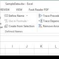 Formula bar in excel reflects
 Changing and aligning fonts in cells How to change the main font in Excel