Excel wrapping by words. Wrap lines in one cell

Different users attach different meanings to the same words. So, by the word string, some understand a string variable, others a set of horizontally oriented cells, and still others a line of text within a cell. In this publication, we will look at line breaks, keeping in mind that the meaning of words can be different.

How to move rows in Excel to a new sheet?

As you know, you can transfer rows from one sheet to another either in one range (when each next row has a common border with the previous one), or only one at a time. All attempts to select several disconnected lines and then cut the selected lines in one action inevitably end with the message "This command is not applicable to disjoint ranges. Select one range and select the command again." Thus, Excel presents the user with the choice of either cutting and pasting rows one at a time, which does not seem like an attractive task, or looking for other ways to solve the problem. One such method is to use an add-in for Excel, which allows you to quickly transfer rows with specified values and satisfying specified conditions to a new sheet.

add-on for conditional line wrapping

The user is given the opportunity to:

1. Quickly call the add-in dialog box with one click on the button located on one of the Excel ribbon tabs;

2. Specify one or several values for search, using ";" as a separator character. semicolon;

3. Consider or ignore case when searching for text values;

4. Use both the used range and any arbitrary sheet range specified by the user as a range of cells to search for specified values;

5. Select one of eight conditions for the cells of the selected range:

a) coincides or does not coincide with the desired value;

b) contains or does not contain the desired value;

c) begins or does not begin with the desired value;

d) ends or does not end with the desired value.

6. Set limits for the selected range using line numbers.

Break a line in a cell

How to move text in a cell to a new line

To move text to a new line within one cell, To transfer text, you must press the key combination Alt+Enter.

How to replace a line break with a space

It is often necessary to get rid of line breaks and remove them in order to bring cell values to their normal form. If you look at the ASCII code table,

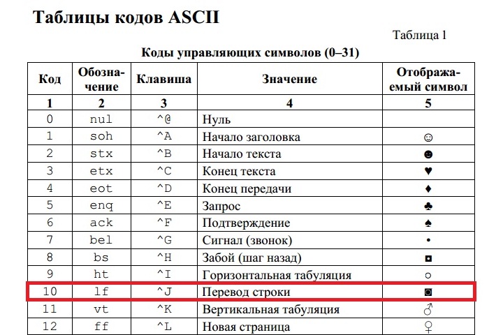
you can see that the application uses code number 10 and the name “Line Feed”, which corresponds to the key combination Ctrl+J. Knowing this, you can remove line breaks using a standard Excel tool such as Find and Replace. To do this, you need to call the dialog box with the Ctrl+F key combination (this field will remain empty), go to the "Replace" tab, place the cursor in the "Find" field, press the Ctrl+J key combination and click the "Replace" or "Replace All" button ". Similarly, you can replace a line break with a space.

It is often necessary to wrap text inside one Excel cell to a new line. That is, move the text along the lines inside one cell as indicated in the picture. If, after entering the first part of the text, you simply press the ENTER key, the cursor will be moved to the next line, but to a different cell, and we need a transfer in the same cell.

This is a very common task and it can be solved very simply - to move text to a new line inside one Excel cell, you need to click ALT+ENTER(hold down the ALT key, then without releasing it, press the ENTER key)

How to Wrap Text on a New Line in Excel Using a Formula

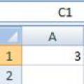
Sometimes you need to make a line break not just once, but using functions in Excel. Like in this example in the figure. We enter the first name, last name and patronymic and it is automatically collected in cell A6

In the window that opens, in the “Alignment” tab, you must check the box next to “Word wrap” as indicated in the picture, otherwise line wraps in Excel will not be displayed correctly using formulas.

How to replace a hyphen in Excel with another character and back using a formula

Can change the hyphen symbol to any other character, for example on a space, using the text function SUBSTITUTE in Excel

Let's take an example of what is in the picture above. So, in cell B1 we write the SUBSTITUTE function:

Code:

SUBSTITUTE(A1,CHAR(10);" ")

A1 is our text with a line break;
CHAR(10) is a line break (we looked at this a little higher in this article);
" " is a space because we are changing the line break to a space

If you need to do the opposite operation - change the space to a hyphen (symbol), then the function will look like this:

Code:

SUBSTITUTE(A1;" ";CHAR(10))

Let me remind you that in order for line breaks to be reflected correctly, you must specify “Wrap across lines” in the cell properties, in the “Alignment” section.

How to change the hyphen to a space and back in Excel using SEARCH - REPLACE

There are times when formulas are inconvenient to use and replacements need to be made quickly. To do this, we will use Search and Replace. Select our text and press CTRL+H, the following window will appear.

If we need to change the line break to a space, then in the “Find” line we need to enter a line break, to do this, go to the “Find” field, then press the ALT key, without releasing it, type 010 on the keyboard - this is the line break code, it is not will be visible in this field.

After that, in the “Replace with” field, enter a space or any other character that you need to change to and click “Replace” or “Replace All”.

By the way, this is implemented more clearly in Word.

If you need to change the line break character to a space, then in the "Find" field you need to indicate a special "Line Break" code, which is denoted as ^l
In the “Replace with:” field, you just need to make a space and click on “Replace” or “Replace All”.

You can change not only line breaks, but also other special characters, to get their corresponding code, you need to click on the “More >>”, “Special” button and select the code you need. Let me remind you that this function is only available in Word; these symbols will not work in Excel.

Quite often the question arises, how to move to another line inside a cell in Excel? This question arises when the text in a cell is too long, or when wrapping is necessary to structure the data. In this case, it may not be convenient to work with tables. Typically, text is transferred using the Enter key. For example, in Microsoft Office Word. But in Microsoft Office Excel, when we press Enter, we go to the adjacent lower cell.

So we need to wrap the text to another line. To transfer, you need to press the keyboard shortcut Alt+Enter. After which the word located on the right side of the cursor will be moved to the next line.

Automatically wrap text in Excel

In Excel, on the Home tab, in the Alignment group, there is a “Text Wrap” button. If you select a cell and click this button, the text in the cell will wrap to a new line automatically depending on the width of the cell. Automatic transfer requires a simple click of a button.

Remove hyphen using function and hyphen symbol

In order to remove the carry, we can use the SUBSTITUTE function.

The function replaces one text with another in the specified cell. In our case, we will replace the space character with a hyphen character.

Formula syntax:

SUBSTITUTE (text; old_text; new_text; [occurrence number])

The final form of the formula:

SUBSTITUTE(A1,CHAR(10), " ")

A1 – cell containing hyphenated text,
CHAR(10) – line break character,
» » – space.

If, on the contrary, we need to insert a hyphen to another line, instead of a space, we will perform this operation in reverse.

SUBSTITUTE(A1; ";CHAR(10))

For the function to work correctly, the “Wrap by words” checkbox must be checked in the Alignment tab (Cell Format).

Transfer using the CONCATENATE formula

To solve our problem, we can use the CONCATENATE formula.

Formula syntax:

CONCATENATE (text1,[text2]…)

We have text in cells A1 and B1. Let's enter the following formula into B3:

CONCATENATE(A1,CHAR(10),B1)

As in the example I gave above, for the function to work correctly, you need to set the “word wrap” checkbox in the properties.

Most Microsoft Excel settings are set by default, including the limitation: one cell - one row. But there are many cases when you need to make several lines in a cell. There are several ways you can do this.

In addition to the arrangement of words in one cell, writing a long word often turns out to be a problem: either part of it is transferred to another line (when using Enter), or it ends up in an adjacent column.

The Excel office product has a varied range of solutions for many tasks. Wrapping a line in an Excel cell is no exception: from manual breaking to automatic wrapping with a given formula and programming.

Using a key combination

In this case, use the keyboard shortcut " Alt+Enter" It will be more convenient for the user to first hold down “Alt”, then, without releasing the key, press “ Enter».

You can move text in a cell using this combination at the time of typing or after all the words are written on one line. You need to place the cursor in front of the desired word and press the specified key combination - this will create a new line in the cell.

When you need to write large text, you can use the command " cell format", which will allow you to fit the text in one Excel cell.

By clicking the mouse highlight required area. Right-click to open a dialog box with commands. Choose " cell format».

On the top panel, select the section “ leveling».

Check the box against the command " translate according to words"(column "display"). Click OK.

After which the dialog box will close. Now the cell is filled with long text, word wrapping will be be carried out automatically. If the word does not fit in width, then Excel itself will wrap the line in the cell.

If there should be several such cells, you need to select them all with the left mouse button and perform the above algorithm of actions. Automatic transfer will appear in the entire selected area.

Using Formulas

When the user needs not only to divide the text into lines, but also to first collect information from several places, then the above methods are not suitable. In this case, several types of word transfer formulas are used:

symbol ();
concatenate();
substitute().

Symbol

Inside brackets the code is indicated– a digital value from 1 to 255. The code is taken from a special table, where the number and the corresponding carry character are indicated. The transfer code is 10. Therefore, the formula used is “character(10)”.

Let's look at a specific example of how to work with the formula “character(10)”. First, let's fill in the cells, which we will later merge. 4 columns of the first line - last name, gender, age, education. The second is Ivanova, female, 30, higher education.

Select, then select a cell, where we will carry out the transfer. Place the cursor in the formula bar.

Filling out the formula(for selected cell):

A1&A2&CHAR(10)&B1&B2&CHAR(10)&C1&C2&CHAR(10)&D1&D2

Where the “&” sign means concatenation of corresponding cells, and the symbol (10) means a line break after each concatenated pair.

After writing the formula, press the " Enter" The result will appear in the highlighted area.

The screenshot shows that the format is not set. We use " string format", as stated above. After the checkbox next to the item “ translate according to words", the cell will look like the picture below.

There is another way to quickly use this command. At the top right there is a section “ Format" Click on the small black arrow to bring up a dialog box. Below is the desired command.

If you replace the original data with others, the contents of the cell will also change.

Couple

The “concatenate()” function is similar to the previous one. It is also given by a formula, but in brackets it is not the code that is indicated, but the formula “character (10)”.

Let's take for example only the first row with 4 columns.

Select the area to be transferred and point the cursor at the formula bar. Let's write down:

CONCATENATE(A1,CHAR(10),B1,CHAR(10),C1,CHAR(10),D1)

Press the key " Enter».

Let's set " translate according to words" We get:

Number of cells for clutch it can be anything.

The main advantage of this method is that changing the data in rows and columns does not change the formula; it will have the same specified algorithm.

Substitute

When a cell contains many words and you need to move them to another place immediately with a transfer, then use the “substitute()” formula.

Enter the required text in A4.

Then select A6 with the left mouse and write it in the formula:

SUBSTITUTE(A4;" ";CHAR(10))

Insert the address of the cell with the text into the formula - A4. After pressing the " Enter"we get the result.

It is important not to forget to check the box next to the command " translate according to words».

Replacing a hyphen with a space and back

Sometimes you need to replace the hyphen with a space and make a column of words a solid text. There are several ways to do this. Let's look at two of them:

window " find and replace»;
VBA scripts.

Find and replace opens with a keyboard shortcut Ctrl+H. For convenience, you first need to hold down the Ctrl key, then press the English letter H. A dialog box with customizable parameters will pop up.

In field " find» should be entered Ctrl+J(first holding down the key, then typing the letter). In this case, the field will remain practically empty (there will be only a barely noticeable blinking dot).

In field " replaced by"You need to put a space (or several), as well as any other character to which you plan to change the hyphen.

The program will highlight the area of the file with the required values. Then you just have to press “ replace everything».

Columns of words will be rearranged into lines with spaces.

Using a VBA script

You can open the editor window using a keyboard shortcut Alt+F11.

In the editor we find the panel “ VBAProject" and click on the file you are looking for. Right-click to open the context menu. First select " Insert", then " Module».

A window appears to insert the code.

We type the code there. If need to replace hyphen space, then we write:

Sub ReplaceSpace() For Each cell In Selection cell.Value = Replace (cell.Value, Chr(32), Chr(10)) Next End Sub

If vice versa:

Sub ReplaceTransfer() For Each cell In Selection cell.Value = Replace (cell.Value, Chr(10), Chr(32)) Next End Sub

Where Chr (10) is the line break code, and Chr (32) is the space code.

A window will pop up where you need to click the “ NO».

Next you need save document with new macro support.

To close the editor, click " Alt+Q».

The main disadvantage of this method is that it requires basic knowledge of the VBA language.

Variable solutions to a problem allows the Microsoft Excel user to choose the method that suits him.

Excel is an extremely functional program; it contains a huge number of functions that a beginner, as well as an experienced user, will have to get acquainted with for a very long time. Earlier I already told you about many of the nuances of Excel, about formulas, functions, etc. This time I will touch on a not very complex, but quite pressing topic regarding how a new row is created in an Excel cell.

You won’t be able to get by with one key, as is the case with other programs, because you will simply jump to a new cell. There is a solution, not just one, but two! But first things first.

Using a keyboard shortcut

The simplest option is to use a key combination on the keyboard specially designed for such purposes. You may not know, but in order to create a new line inside one cell, you just need to simultaneously hold down the same notorious and . But this option is only suitable in cases where you perform such a one-time operation. Otherwise, it is more advisable to use the formula, which will be discussed below.

Using formula

It also happens that the above action is not enough. For example, imagine a situation where we first need to connect adjacent cells, and then write down all the information from each line, but within one cell. In the screenshot you see the initial data and the result you need to achieve.

So, let's do the following:

A1 and B1, A2 and B2, A3 and B3 (A1&B1, etc.).
Next, using a special line break code. Here I will make a reservation that there is a special table where each sign means some action. The line break code is 10, and the complete function will look like this: “CHAR(10). Based on the above, in cell A6 we must write the following: A1&B1&CHARACTER(10)&A2&B2&CHARACTER(10)&A3&B3.

In some cases, line breaks will not be displayed entirely correctly, so to be on the safe side, I recommend doing this.