How to combine cells in Excel without data loss. Practical Tips - How to Combine Cells in Excel
IN office package MS Excel can be combined with several fields adjacent horizontally or vertical in one large. This can be done by several methods.
Use the context menu
Calling right key Mice context menu, after selecting fields requiring merge, you should select Format.
We are interested in tab Alignment.
In the property Display Let's notice tick An association and click OK.
Should be consideredThat the combined field will save only the value of the top left. 
Button on the tape for Excel 2007 and above
You can also use the ribbon button to merge.
IN version of Office. 2013 it is located on the tab the main And looks like this.


By default button unites and produces alignment Text in the center. In the drop-down list, among the proposed options, there is also a row association, without alignment and cancelIf you change your mind. The same button can split them back.
Before pressing this button follows highlight Range of vertical or horizontal cells.
In Office 2010, the button has an almost the same look with a similar drop-down list. 
In Office 2003, the combination button with a similar function is on the toolbar Formatting.
Clear cells can be used copyPaster, i.e copy (Ctrl + C) combined, after which insert (Ctrl + V) it in the desired place. 
Use the "Capture" function
Excel has a feature Tie. Combines several lines into one. 
In the function itself Tie It follows through the point with the comma to specify the cells you need or range:
\u003d Catch (IR1; Ball2; ...) From 1 to 255 function arguments.
A similar clutch procedure can be made in this way:
We write macros
You can write a simple macro (or use for these purposes. macrorecorder) and appoint him some convenient for you combination of hot keys. Possible options for such a macro are presented below.
The second option will ensure the combination with the preservation of the initial these all combined fields. 
Select the necessary fields and execute the macro. Editor VBA. opens a combination Alt + F11.
We introduce Macro software code and perform. 
To start the created macro, click Alt + F8.. The window will start Macro (Macro). In the list Macro name (Macro Name) Select the desired and click Perform (RUN). 
How to combine columns
In Excel, you can combine values two columns in one line. For example, we want to combine the document and information about it. 
This can be done as follows. Allocate first column, then on the tab the main — Editing Click on the field Find and highlight, in the list of interest " Select a group of cells ...«: 
In the window that opens, put a tick - Empty cells, then OK.
In the second column there are empty columns - highlight them. 
After the sign equal to enter formula The values \u200b\u200bof the corresponding field of the desired column: 
Then Ctrl + Enter. And the values \u200b\u200bare standing only in the empty cells of the second column. 
How to combine cells with hot keys
By default, such a combination does not existHowever, you can do this: select the required cells, combine the button on the tape.
With any subsequent selection, press F.4 (Repeat the last team!).
Also in the settings you can assign a desired combination for the desired command at discretion, or write a macro (for more advanced users) for these purposes).
When placing tables for a more visible display of information, there is a need to combine several cells in one. This is often used for example when specifying one common data header that have different values. An example of such a display of information you can see in the image below. About how to combine cells in Excel are step by step read further. You can combine not only horizontally, it is possible to combine vertical, as well as groups of horizontal and vertical cells.
An example of a discharge combining with one discharge header and different data
How to combine cells in Excel
To combine cells, you can use in two ways. The first is with the help context menu through the format. Highlight all the cells that you want to combine and click on the allocated area right-click. In the drop-down context menu, select "Cell format ...".

In the format window, go to the "Alignment" tab and in the Display unit, check the checkbox "Customs" checkbox.

Mark the "Customs Union" item in the Alignment tab
If there are any data in the cells, Excel issues a loss warning every time in addition to the top left. Therefore, be careful when combining and do not lose important data. If you still need to combine the cells with the data, agree by clicking OK.

In my case, only the number "1" from the left upper cell remains out of the 10 numbers in the combined cells.

By default, Excel after the union aligns the data on the right edge. If you need to quickly merge and at the same time immediately align the data in the center, you can use the second way.
As in the previous method, select the cells that need to be combined. At the top of the program in the "Home" tab, find a block called alignment. This block has a drop-down list that allows you to combine cells. For the union there are three types:
- Combine and place in the center - the result of clicking on this item will be exactly the same merging as in the previous example, but Excel formats the alignment of the resulting data in the center.
- Combine by lines - if the area of \u200b\u200bcells with several lines is highlighted, the program will bring together line and in the event that the data is present, will only leave those that were in the left.
- Combine cells - this item acts in the same way as in the first embodiment through the format.
- Cancel Association - You need to select a cell that was previously combined and click on the menu item - the program will restore the structure of the cells as before the union. The data before the union will naturally not restore.
Having tried any of the ways, you will know how to combine cells in Excel.

The second way to quickly unite cells
The Excel document structure is strictly defined and so that there are no problems and errors in the future with calculations and formulas, in the program, each block of data (cell) must match the unique "address". The address is an alphanumeric numerical designation of the column and string. Accordingly, one column must only correspond to the lines cell. Accordingly, divided the previously created cell to two will not work. To have a divided into two cells, we need to think about the table structure in advance. In the column where the separation is necessary to schedule two columns and combine all cells with data where there is no separation. In the table it looks like this.

It is not possible to divide the cell in Excele. One can only schedule the structure of the table when creating.
In line 4, I have a divided into two cells. For this, I planned two columns "B" and "C" for this column. Then in lines, where I do not need the separation, I combined the line of the cells, and left in line 4 without united. As a result, the table contains the "section" column with the two cell divided into the 4th line. With this way of creating separation, each cell has its own unique "address" and can be applied to it in the formulas and addressing.

Now you know how to smash the cell in Excel for two and you can plan the structure of the table in advance to then do not break the table already created.
In the previous article, I described an example of creating a simple table with computing. Now we will analyze which operations can be performed on cells in the spreadsheet. Consider the following steps: Combine and separating the cells, resizing and location of data inside the cell, as well as protection of the formula or content from change.
How to combine cells in Excel
The combination operation may be required if it is necessary to display data from the overlap of several columns - the name of the column group.
Check out the example below. Celling was used to center the table name.
To perform this operation, it is necessary to select cells occupy the desired width and in the tape tape on the tab the main In chapter Alignment Click button Combine and put in the center.
Calling button for connecting cellsIn the process of combining several adjacent cells horizontally or vertical, they are transformed into one large cell, which occupies the width of the selected columns or the height of the selected lines.
Important!After the combination, the data is displayed only by one cell, which were in an extreme left upper cell of the selected range. The contents of other integrated cells will be lost.
The result of the combination can be canceled by returning the previous number of cells. To do this, click on the desired cell and press the button that was used to combine (see above). Cells will be divided. At the same time, the data will be recorded in the extreme left cell.
Tip! If you often perform the same operation, then it does not click on the menu each time, press the button F4. On your keyboard. This is a quick challenge of the last used command.
Look at the short video below
How to combine cells in exile with text preservation
The problem of data loss when combining cells has already been mentioned above. So is there a way to save this data? There are many options. But in each of its troubles and better knowledge. You can perform this. I wrote about them in previous articles. You can use macros, but all this for advanced users. I suggest easy enough, but effective method. It will save data from cells.
The following describes operations using hot keys Ctrl + C. -coping, Ctrl + V. - Box
1 option We combine the text in one line
- Select cells with the desired data and copy the contents of Ctrl + C.
- Open a notepad program ( text editor) And insert the CTRL + V copied into it.
- What was inserted into the notebook, we allocate and reinstate Ctrl + C.
- Go to Excel. Remove data from source cells. Click on the first. After clicking in the formula string (highlighted with an orange rectangle in the figure below) and press Ctrl + v.
Why insert the formulas in the formula row? Because the tanning signs are saved in the notebook. And when inserted directly to the table, the data will again break through different cells.
Option 2 We combine the text in line in several lines
- Repeat items 1 and 2 from the previous version
- Now delete tabs in notepad. Highlight the emptiness (interval) between any words. Copy its Ctrl + C.
- In the notepad menu, select Edit - replace. Click in the field that: and press Ctrl + V. You insert an invisible tab of the tab.
- Click in the field than: and press the Space key. Next, replace everything button.
- We allocate and copy all the text from the notepad
- Go to Excel. Remove data from source cells. Click on the first. And insert the data Ctrl + V
The data will be inserted on rows with text union in each.
 Combining cells in Excel with text preservation
 How to find combined cells
If you have to adjust the sheet with a multitude of combined cells, then manually do it too tiring. We use the search tool to find such cells.
On the Home tab, in the Edit section, click the button. To find (magnifying glass icon) or use key combination Ctrl + F.. The following window opens (see below).
Press the button Format (highlighted in a red rectangle)
 Schedule search window
 The window will open in which go to the tab Alignment and set the checkbox in the section Display At paragraph Combining cells
 Find a window format
 Press OK. And in the next window we see the result of the search.
 List of found combined cells
 Now, clicking at the address of the cells in the search results (highlighted by a red frame), it will allocate to Sheet spreadsheet.
How to divide the cell in exile
Unfortunately, Excel cannot be broken down as it is done in table Word.. But here you can schitrate - add empty cells and combine cells from above to get the look divided. To do this, highlight the cell or group of cells to insert the same amount of new ones. Click on highlighting the right mouse button and select the Paste action from the context menu. Next, choose what and how to insert (see the picture below)
 The result of inserting the group of cells with a shift to the right
 By the way, in the same way you can delete one or group of cells.
When creating a new book or sheet, the table has the same cell sizes, but maybe these sizes will not meet our requirements. And then they should be changed.
The width of the columns in Excel is set by a numerical value that corresponds to the number of freely displayed characters. By default, this value is 8 characters with a tail. And the height of the rows is set in points as the font size, and the default is 12.75.
There are several ways to consider them. First, it is necessary to select cells (rows or columns), the size of which should be changed.
1 way. Change the mouse
When you hover the mouse pointer in the zone of column names or lines numbers, the cursor takes the form of a bidirectional arrow. If at this moment to hold left button Mouse and continue moving, then a change in the position of the cell's border will be changed. And this change will reflect on all allocated.
 Changing the width and height of the cell with a mouse
 2 way. Change the command from the menu Format
In the tape tape on the tab the main In chapter Cells Click button Format and in the drop-down list choose the right action Column width or String height.
 Install the sizes of the cell
 We specify the desired values \u200b\u200band the dimensions of the selected cells will become the same.
Attention! If the column width is insufficient to display numeric data, instead of numbers will be visible signs ### . In this case, the width value should be increased.
How to make a word transfer in Excel Cell
When filling the tables of the table of data, they are displayed in one line, which is not always convenient. So part of the data may be hidden due to the insufficient width. But if you increase the height of the cell and place data into several lines, you can get a complete display of the contents and with a small column width. To do this, highlight the desired cells and give the team Format - cell format. In the properties window, we set the parameters (highlighted with red rectangles) as in the figure
 Display text data in a cell in several lines
 You can forcibly divide the enabled data into several lines. To do this, you need to press the key combination Alt + Enter..
How to Protect Cells from Editing
If it is assumed that other users will work with your table, then you can block cells containing formulas from random or deliberate change. To block, you must enable sheet protection.
By default, all cells are marked as protected, and after turning on the leaf protection, change their contents will not be possible. Therefore, you first need to define cells that will be available to change after installing protection. To do this, select the cell or group of cells, go to the menu Cell format And on the tab Protection Remove the checkbox from the point Protected cell..
 Change Cell Protection
 The second option quickly remove or remove the cell protection property - this is the choice of the team Block the cell either from the menu Format On the tab the main.
After specifying the protected cells, we go to the tab Review And give a team Protect sheet. In the next window, set the password and additional permissions that can be performed with this sheet. Next click OK.
 Installation of sheet protection
 Attention! If you forget the password, you will not be able to edit secure cells. If you leave the password field blank, then the protection can disable any user.
Now when you try to change data in a secure cell, the user will see the following warning
 Data protection warning from change
 To remove the protection, you must enter a password in response to the command. Review - Remove Leaf Protection.
Dear reader! You looked at the article to the end.
Did you get the answer to your question? Write in the comments a few words.
If the answer was not found, specify what was looking for.
The need to combine cells in Excel arises from the user quite often. It would seem that here is this, because there are many ways to make it enough. However, users, especially those who are accustomed to working with Word, it is important to remember about one very an important moment: When combining cells, only the value that is located in the upper and left cell remains. As for the rest of the data, they simply will be erased.
If you are upset at this stage, I want to delight you: there is still a way out, and not one! Actually, this material I would like to devote to the question regarding how the cells are associated in Excel without losing data.
How to combine cells
However, before I tell you about it, I would also like to mention the ways to combine cells when the data is not yet made or if their disappearance does not greatly upset. Nevertheless, there are quite a few users who want to enlighten and in this matter including.

How to combine cells without losing data
Here I, perhaps, also allocate two ways to do this:
- The first is to use the add-on, let it be VBA-Excel. After you download this product and install it, an additional "Combine cells" will appear in the main tape of the program. Accordingly, for this you need to simply highlight them, after which you specify the desired word separator: point, comma, point with a comma or a row transfer.
- The second way is simpler and consists in using the built-in excel. Once I already told how to use it, but I repeat briefly again: call the "Wizard of Functions", then start tying the name. In the "Function Arguments" window for the "Text 1" field, select the first cell among those that need to be combined with the left mouse button. In the "Text 2" field, select the next cell and so while they are not running out. Please note that immediately the entire range of cells cannot be combined, they must be separated by a semicolon. For example, your formula may look like this: \u003d Catch (A1; B1; C1).
Well, it seems nothing complicated. Now and you know how to combine unfilled cells and how to do the same with cells whose data cannot be lost categorically!
Video to help
Users only begin to work with Excel table editor, often arises how to combine cells in Excel.
For this, there are special commands and functions in the program itself, as well as several ways of type of superstructure and macros.
All of them are simple enough to learn how to use for just a couple of techniques, using the following tips.
Using standard Excel functions, you can combine table cells.
At the same time, they are aligned in the center, connected by lines or simply combined with the remaining of former formatting.
Tip! It is best to carry out in advance, with even empty cells, since after the procedure information remains only in the extreme left cell on top.
Combining through the context menu
The easiest I. fast way Combine cells and write data into one enlarged column and the string is to use the context menu.
The order of action is as follows:
- There is a range of cells that require association;
- On the selected part of the table, the right mouse button is pressed;
- In the menu that opens, the "Format of the cells" is selected;
- The Alignment Tab opens;
- A check mark opposite the "combining cells".
The method is simple, but suitable, naturally, only for text data - cells with numbers and formulas to combine unacceptably and meaningless.
It is worth noting that in this case, only information remains in the combined area from its left upper part, which the program warns in advance.

You can save data by coping them in advance to another area, and after combining to attach to the remaining text
Union through the toolbar
For type and older versions, the combination icon is displayed immediately into the panel. By clicking it, you can not only quickly connect areas, but immediately align them in the middle.
This is done to accelerate the formation process in the text header string, which are often created in this way.
If the execution of the command led to the central location of the data that is not required for the text, they are easy to set them to the desired position (left or right) using the alignment commands.
In the Excel 2007/2010/2013 panel, this button is also there, on the Home tab (group "Alignment").
However, it is already equipped with a drop-down menu to increase the number of actions performed with its help.

Using the given commands, you can simply combine the elements of the table with the central alignment, but also execute two additional options for:
- Create a whole group of combined cell rows;
- Combine without setting text in the center.
Combine columns are not even in this version.
Sometimes the area cannot be merged, and the buttons and commands remain inactive. This happens if protection or book (document) is installed on the sheet (document) only general access.
Before connecting areas, you must remove all these conditions by opening the ability to format the table.
Function for text combining
In order for the merger to happen without loss important information And the data did not have to distribute on other cells and return it back after the union, it is worth using the "Capture" function.
Make it easy:
- First, the cell is selected near the united areas and is formatted in the desired way (for example, it is made in size 3x3 or 2x6);
- It is written in the type formula (A1; A2), where the cells are specified (one!), The text of which will be combined).

The result will be the combined field of the type:

Information in the area D1: F8 from cells A1 and C3, connected without loss of text
 How to combine two accounts on Facebook?
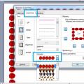 Download and insert a beautiful framework to Word Document
 How to fix clock_watchdog_timeout type "Blue screen" (0x00000101)